Show case (FABP4_workflow)

This workflow correspond to the “Show case” section in the VDS Scipion-chem publication. In this example, a bigger dataset extracted from the database DUD-E is used to validate our workflow engine. The specific dataset used is FABP4 , corresponding to the PDB structure 2NNQ). The files contained the receptor structure plus an original set of 47 active molecules and around 50 decoys per active, accounting for a total of 2749 decoy molecules.

As described in the paper, a similar workflow than the one used for 4ERF is run over this new, bigger dataset, as an example of Scipion-chem and to validate its VDS tools. Below, we will explain step by step the protocols contained in this workflow, together with their corresponding inputs, outputs and intermediate viewers.

1. Import

   The initial receptor and ligand structures can be imported in several ways, as we explained in the previous workflow. In this example, we imported the structures directly from the pdb files (for the receptor, corresponding to PDB 2NNQ) and sdf files (for the ligands) files provided by DUD-E. The forms provided by Scipion (in the images below) allow the user to choose the origin of the structure and, in the case of the small molecules, the molecule handler (RDKit or OpenBabel) to use and if a 3D reconstruction is needed.

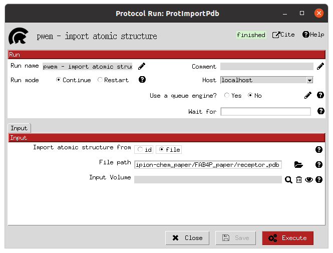
Import receptor form

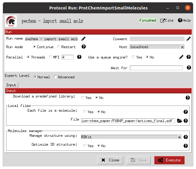
Import active molecules form

2. Preparation

   Once the structures are imported into the Scipion workflow, separate preparation steps are performed for the receptor and the ligand libraries. In this case, we used the protein preparation protocol in the OpenMM plugin, which uses PDBFixer for the receptor protein; and RDKit for the preparation of the ligands. In each of the forms, the user is asked about the preparation parameters desired, such as to removing undesired atoms (waters and other non-protein entities) or reconstructing missing atoms in the receptor; or which force fields to use and whether to generate conformers in the parametrization of the ligands.

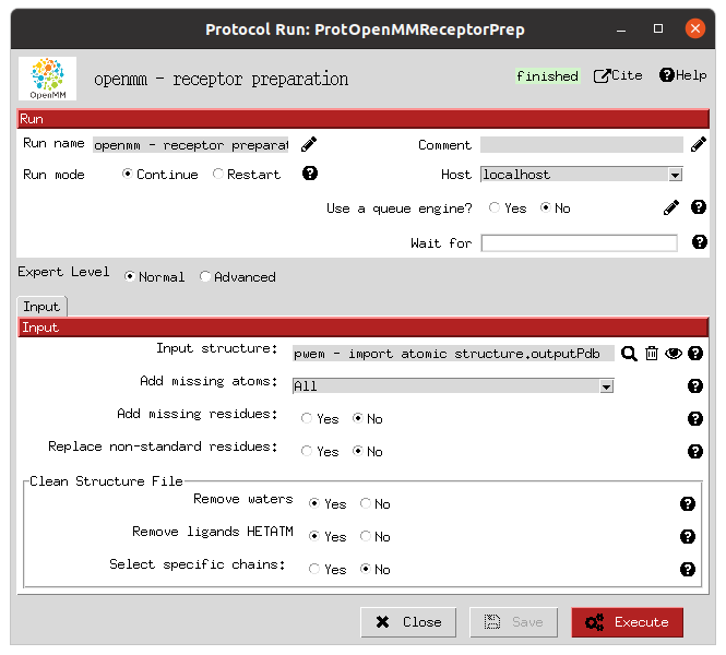
Receptor preparation form

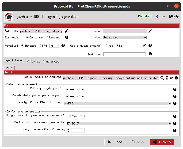
Ligands preparation form

3. ROI definition

   In this particular example, P2Rank is used to predict the most promising pockets in our receptor, which will become those ROIs where we will direct the docking processes. In this step, the main P2Rank protocol is followed by a filter protocol to extract only the 2 best pockets predicted, in order to speed up the downstream workflow. The forms for both protocols are shown, where the corresponding parameters are defined.

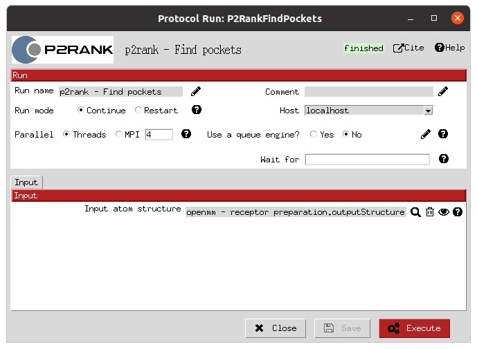
P2Rank ROI prediction form

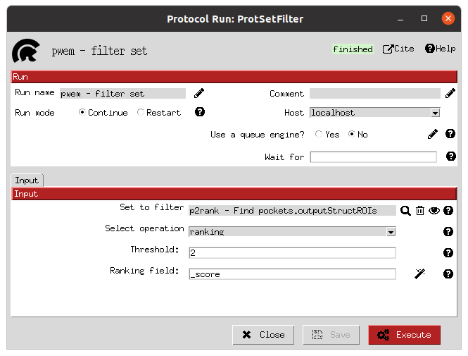
Filter top 2 predicted ROIs form

4. Ligand-based filtering

   On the ligands side, a first filtering step is used by passing 1 ligand-based filter protocol to our active and decoy molecules. This is the ADME filter, which we described in the previous section. The parameters defined in the form determine the specific rules to follow in ADME execution.

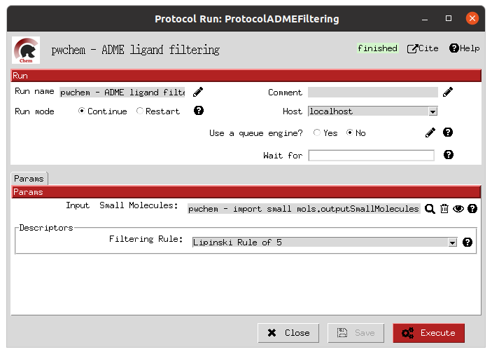
ADME ligand-based filter form

5. Docking

   This steps involves the execution of 3 independent docking programs (AutoDock-GPU, AutoDock Vina and LeDock) over the 2 defined ROIs and both the active and decoy prepared libraries. In practise, this is the slowest step of the workflow, and therefore becomes the usual bottleneck in its execution, so it is important to choose appropriate resources for them. In our case, the forms allow us to define the number of threads and GPUs (only for AutoDock-GPU) to allocate for each of them. Moreover, as the previous cases, the forms also include the parameters that the user can tweak to define the docking processes, such as the number of docking poses to generate for each of the molecule conformers.

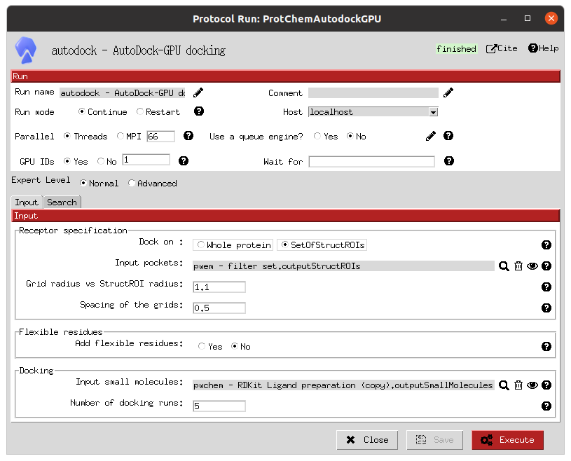
AutoDock-GPU docking form

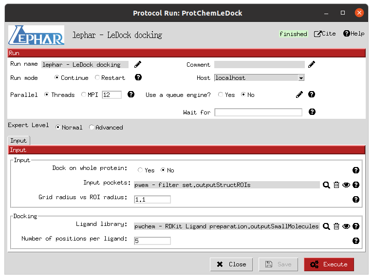
LeDock docking form

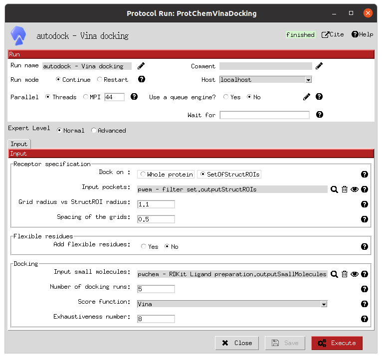
Vina docking form

6. Rescoring

   In order to combine and compare the docking poses generated by each of the software, we need to first evaluate those poses using the same scoring function. In this case, we use the ODDT score protocol to rescore all the docking poses with its Vina score function.

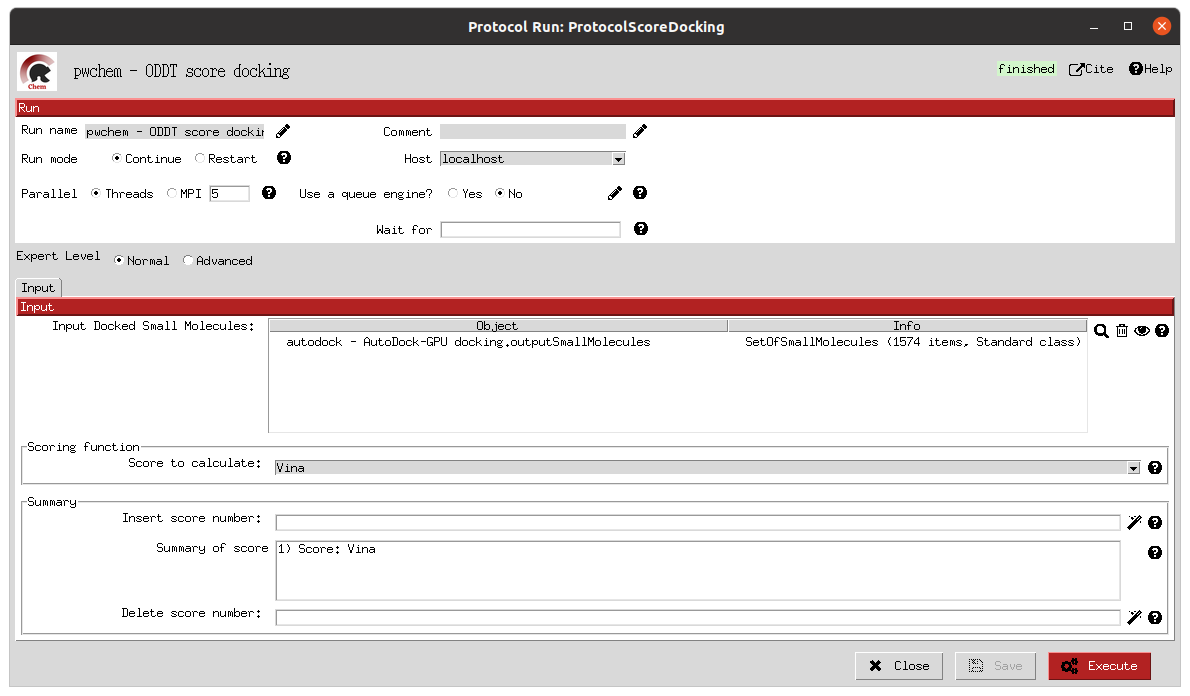
ODDT docking rescoring form

7. Filter and consensus

   Finally, the rescored poses can be combined, ranked and the consensus protocol can be applied to cluster and extract the most promising docking positions. The forms shown below refer to the filter and consensus protocols and their parameters, which are described below. In our example, different combinations of ranking filters and consensus parameters were used in order to evaluate the results. Nine different filtered subsets of our docked molecules containing the 0.01, 0.05, 0.1, 0.5, 1, 5, 10, 50 and 100 % of the highest scored poses were generated to be used in the consensus protocol. Then, for each of these subsets, 2 consensus protocols were executed with a difference in a vital parameter. First, both consensus runs will produce the same pose clusters; however, one of the consensus executions will only consider sufficient those clusters containing at least one pose from each of the 3 docking software (N3) while the other, more permissive one, will consider sufficient those that contain at least poses from 2 docking software (N2). This way, we intend to generate sets enriched in active molecules and smaller than the original set of 2796 molecules.

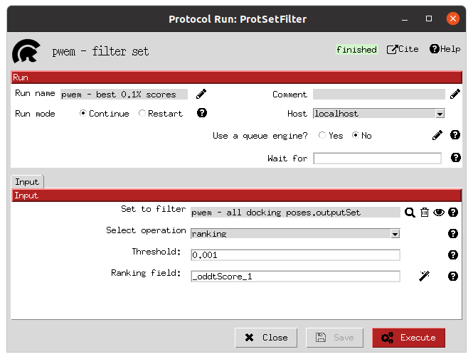
Top scoring filter form

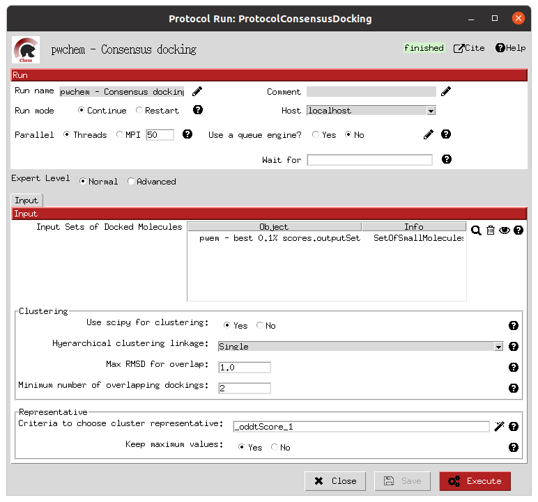
Consensus docking form

The results of this experiment comparing the filtering vs N2 consensus are contained in Fig. ref{fig:ConsResN2}, where we can observe the enrichment of actives vs decoys of the output subsets and the total number of molecules kept for each of them. Subsets labeled %x show the enrichment for the sets generated only passing the score-filter, while those labeled %x_N2 represents the corresponding set generated after passing the score filter plus consensus protocol. A similar image with the results for the N3 consensus, which gave similar results, can be found in the supplementary material.

As we can infer from the graphs, both strategies lead to a considerable enrichment of the original dataset as the percentage of actives (blue bars) is generally enhanced, while the number of total molecules in the subset (red line) is reduced. For our FABP4 example, from the original 2796 (47 actives to 2749 decoys) molecules (1.68% of actives); we got considerable enrichment in both the filtered and filter plus consensus subsets. For instance, we obtained a subset of 64 molecules where 11 actives were kept (17.19%) for the 0.1% filtered subset or, once this same subset is passed through the N2 consensus, we further enriched it to keep 7 actives out of just 24 molecules (29.17%).

Therefore, we were able to reduce the total number of molecules of the original set while significantly enhancing the proportion of actives. However, the user must be careful not to reduce too much the number of docking poses with the score filter since we can observe that subsets below 0.05% lose all or most of the active molecules.

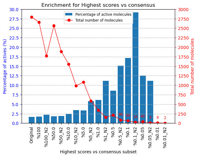
Scipion-chem consensus N2 protocol enrichment. The graph shows the percentage of actives (in blue bars) and the total number of molecules (red dots) for each of the subsets generated in the workflow. The subset ‘Original’ represents the original set imported from DUD-E; ‘%100’ the subset of molecules remaining after the described ligand-based filtering (which slightly improves the enrichment) and then each of the consensus subset generated by applying a best ODDT score ranking filter for the top %x and consensus docking with parameter N2.

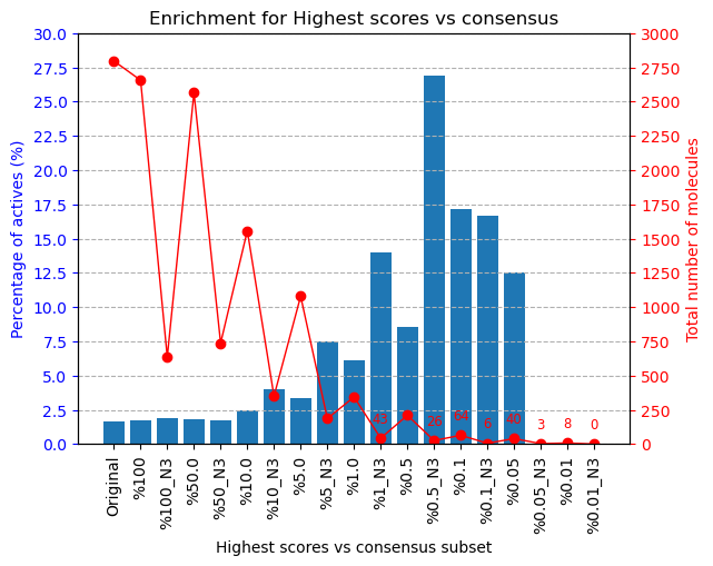
Suplementary Scipion-chem consensus N3 protocol enrichment. The graph shows the percentage of actives (in blue bars) and the total number of molecules (red dots) for each of the subsets generated in the workflow. The subset ‘Original’ represents the original set imported from DUD-E; ‘%100’ the subset of molecules remaining after the described ligand-based filtering (which slightly improves the enrichment) and then each of the consensus subset generated by applying a best ODDT score ranking filter for the top %x and consensus docking with parameter N3.

Additionally, the figure below represents the experimental values for the interaction of the active molecules and the receptor. Each of the points represent an active molecule, placed depending on their experimental value (either Ki in blue or IC50 in red) and their best pose ODDTScore. Those points with a yellow star correspond to the active molecules present in the best resulting consensus dataset (%0.1_N2). As we can observe, the ODDTScore seems to correlate relatively well, and most of the highest ODDTScores represent the best experimental affinities, which are captured in the consensus.

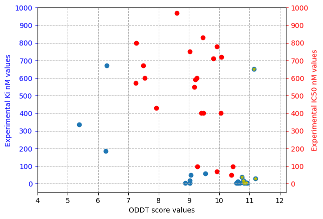
Experimental values of actives against ODDTScore. Yellow stars specify actives found in the best consensus set.